Tutorial 3: the band structure of ZnO (calculated with explicit k-points)
In this tutorial we will calculate the band structure of bulk zinc oxide using the k-space formulation of Koopmans. The input file for this tutorial can be downloaded here.
Calculating the Koopmans band structure
The input file
First, let us inspect the workflow block in the input file:
 2    "workflow": {
 3        "task": "singlepoint",
 4        "functional": "ki",
 5        "base_functional": "lda",
 6        "method": "dfpt",
 7        "init_orbitals": "mlwfs",
 8        "calculate_alpha" : false,
 9        "alpha_guess": [[0.3580, 0.3641, 0.3640, 0.3641, 0.3571, 0.3577, 0.3577, 0.3573, 0.3573, 0.3580, 0.3641, 0.3640, 0.3641, 0.3571, 0.3577, 0.3577, 0.3573, 0.3573, 0.2158, 0.2323, 0.2344, 0.2343, 0.2158, 0.2323, 0.2344, 0.2343, 0.2231, 0.2231]],
10        "pseudo_library": "PseudoDojo/0.4/LDA/SR/standard/upf",
11        "gb_correction" : true,
12        "eps_inf": 5.3
13    },
14    "engine": {
15        "from_scratch": true,
Here we tell the code to calculate the KI bandstructure using the DFPT primitive cell approach. We will not actually calculate the screening parameters in this tutorial (because this calculation takes a bit of time) so we have set calculate_alpha to False and we have provided some pre-computed screening parameters in the alpha_guess field.
The rest of the file contains the atomic coordinates, k-point configuration, and calculator parameters (including the Wannier projectors, which we will discuss later).
Running the calculation
Running koopmans run zno.json should produce an output with each of the steps of the workflow. In particular, there is the Wannierization:
Wannierize
✅
01-scfcompleted✅
02-nscfcompletedWannierize Block 1
✅
01-wannier90_preproccompleted✅
02-pw2wannier90completed✅
03-wannier90completed
Wannierize Block 2
✅
01-wannier90_preproccompleted✅
02-pw2wannier90completed✅
03-wannier90completed
Wannierize Block 3
✅
01-wannier90_preproccompleted✅
02-pw2wannier90completed✅
03-wannier90completed
Wannierize Block 4
✅
01-wannier90_preproccompleted✅
02-pw2wannier90completed✅
03-wannier90completed
Wannierize Block 5
✅
01-wannier90_preproccompleted✅
02-pw2wannier90completed✅
03-wannier90completed
✅
08-merge_occ_wannier_hamiltoniancompleted✅
09-merge_occ_wannier_ucompleted✅
10-merge_occ_wannier_centerscompleted✅
11-bandscompleted✅
12-projwfccompleted
which is very similar to what we saw for silicon, except now we have several blocks for the occupied manifold (discussed below). Then we have
✅
02-wann2kccompleted
where the Wannier90 files are converted into a format readable by the kcw.x code.
If we had instructed the code to calculate the alpha parameters, this would be followed by an extra block where these are calculated. But since we have already provided these, the workflow progresses immediately to the final step
✅
03-kc_hamcompleted
where the Koopmans Hamiltonian is constructed, and the band structure computed.
Plotting the results
Running the workflow will have produced several directories containing various input and output Quantum ESPRESSO files. It will also have generated png band structure plots, including this one of the Koopmans band structure:
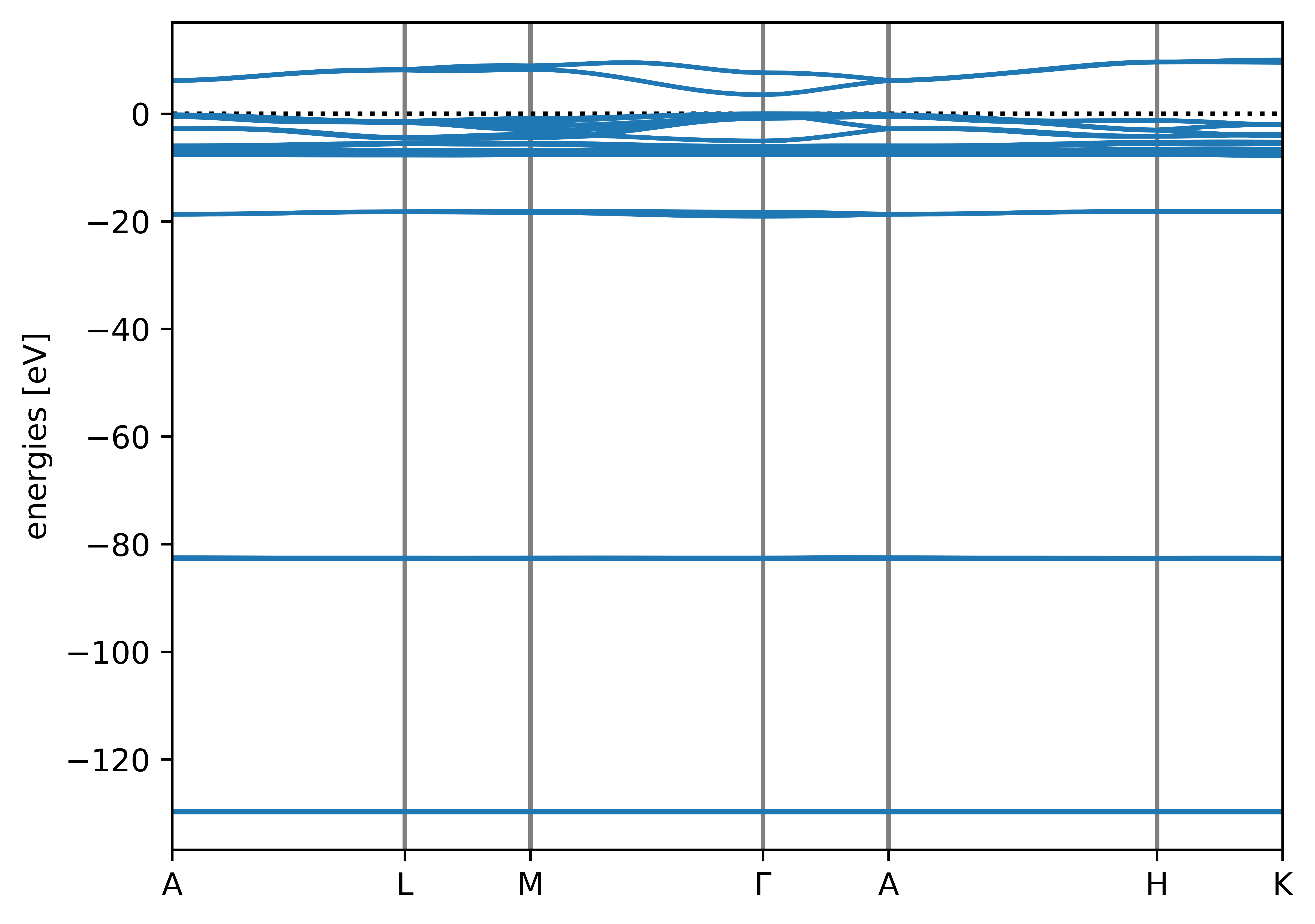
The autogenerated band structure plot for ZnO
However, suppose we want to make a nicer, more comprehensive plot comparing the LDA and Koopmans band structures. To achieve this, we will load all of the information from the zno.pkl file. This will provide us with a SinglepointWorkflow object which contains all of the calculations and their associated results. For example, we can access the calculations corresponding to the Koopmans and LDA band structures as follows:
import numpy as np

from koopmans.io import read

# Load the workflow
wf = read('zno.pkl')

# The Koopmans bands were generated by the very last calculation in the workflow
koopmans_calc = wf.calculations[-1]
and then the band structures are in the results dictionary of these calculators:
[lda_calc] = [c for c in wf.calculations if c.parameters.get('calculation', None) == 'bands']

# Fetch the Koopmans bands, and shift them so that the valence band maximum is zero
koopmans_bs = koopmans_calc.results['band structure']
koopmans_bs_shifted = koopmans_bs.subtract_reference()

# Fetch the LDA bands, and shift them by the same amount
These band structures are BandStructure objects (documented here). Among other things, this class implements a plot function that allows us to plot them on the same set of axes:
lda_bs_shifted = lda_bs.subtract_reference(koopmans_bs.reference)

# Plot the two band structures
With a few further aesthetic tweaks (download the full script here) we obtain the following plot:
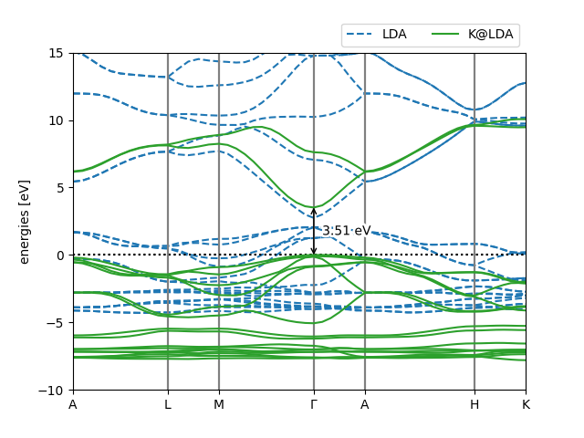
Pretty band structure plot comparing the LDA and Koopmans band structures of ZnO
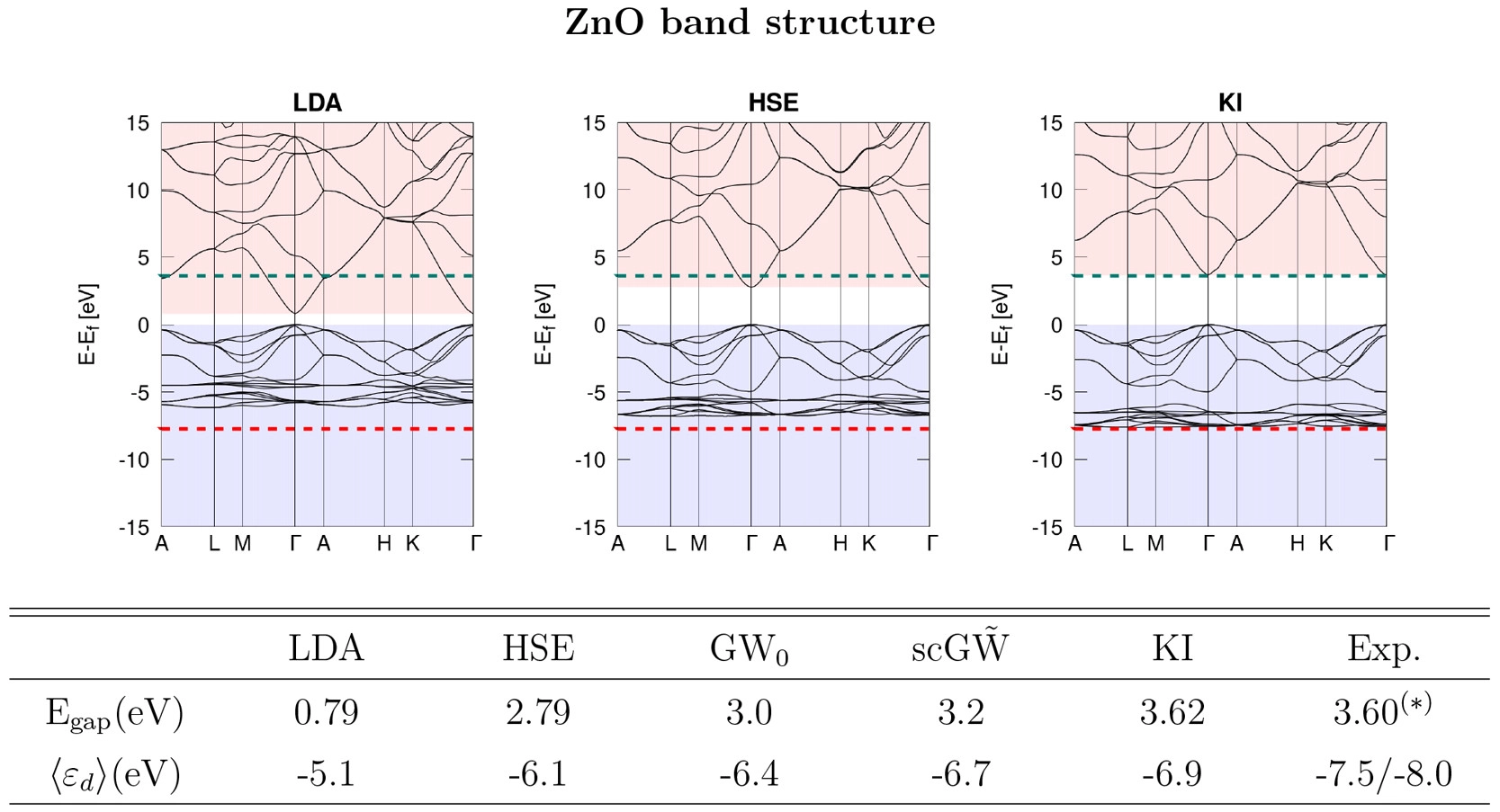
This script has also labelled the band gap for us, which is 3.55 eV. This is pretty close to the 3.62 eV result from Ref. [6] (see the below figure). The slight discrepancy comes from the fact that this tutorial has used coarser parameters to make the calculations run quickly.
Bonus material: understanding the Wannier projections
The first step to any calculation on a periodic system is to obtain a good set of Wannier functions. These depend strongly on our choice of the projections, which (for the moment) we must specify manually.
In the above calculation we gave you some Wannier projections to use:
47    "calculator_parameters": {
48        "ecutwfc": 50.0,
49        "pw": {
50            "system": {
51                "nbnd": 52
52            }
53        },
54        "w90": {
55            "projections": [
But what if you need to come up with your own Wannier projections? In this bonus section we will explain how to work out Wannier projections for yourself.
Configuring the Wannierization
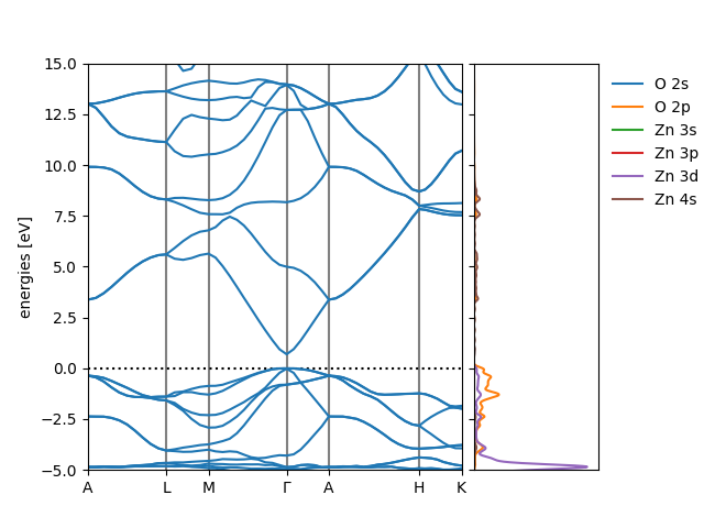
To determine a good choice for the Wannier projections, we can first calculate a projected density of states (pDOS). Take your input file and change the task from singlepoint to dft_bands, and then run koopmans run zno.json (for the sake of tidiness, this input file can be found in the 02-dft_bands directory). This will run the DFT bandstructure workflow, which will produce various files, including a png of the bandstructure and pDOS. If you look at this file, you will see that the DFT band structure of ZnO consists of several sets of bands, each well-separated in energy space:
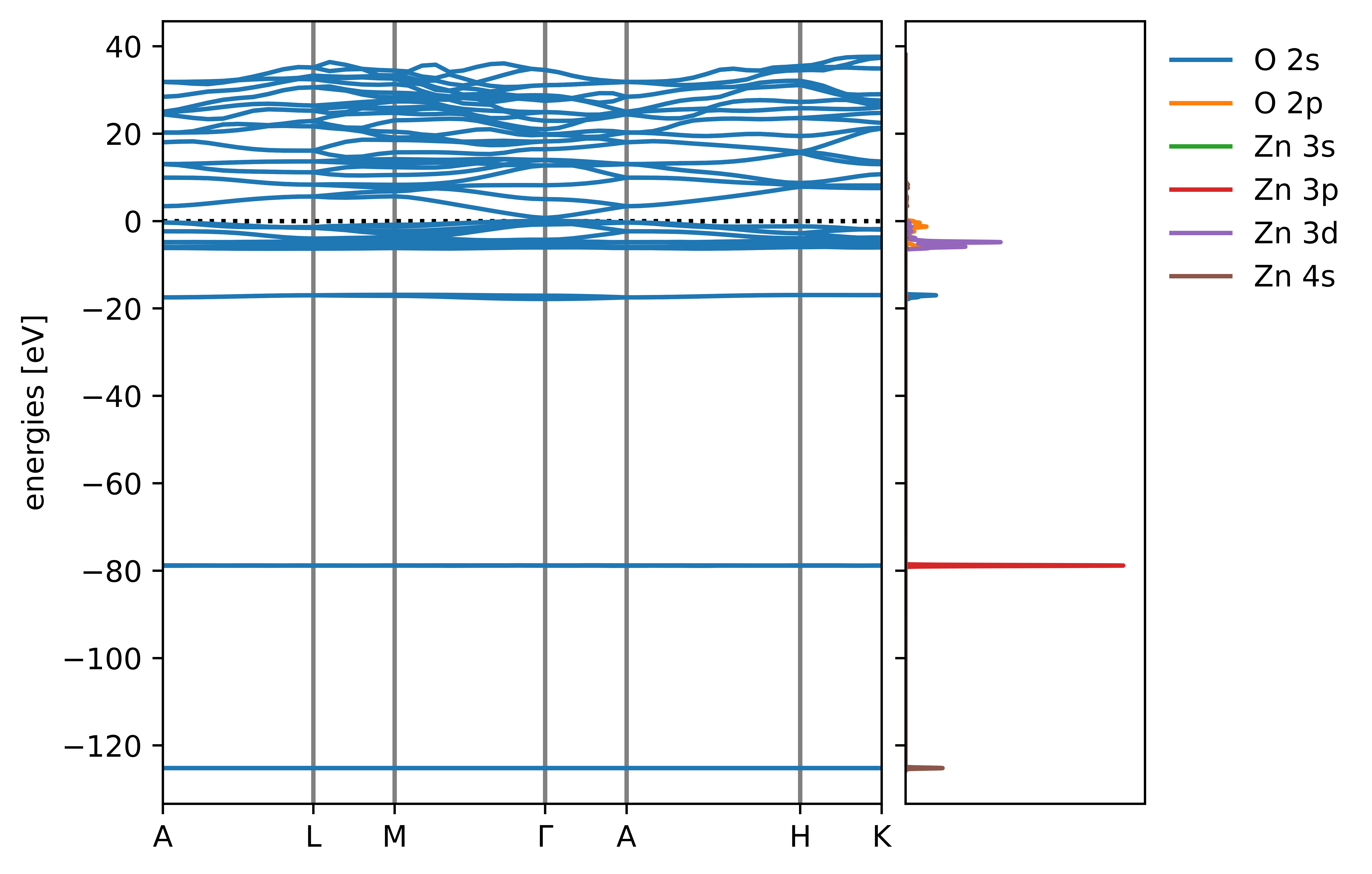
The pDOS of ZnO
As the pDOS shows us, the filled bands correspond to zinc 3s, zinc 3p, oxygen 2s, and then zinc 3d hybridized with oxygen 2p. Meanwhile, the lowest empty bands correspond to Zn 4s bands. A sensible choice for the occupied projectors is therefore
"w90": {
   "projections": [
       [{"site": "Zn", "ang_mtm": "l=0"}],
       [{"site": "Zn", "ang_mtm": "l=1"}],
       [{"site": "O", "ang_mtm": "l=0"}],
       [{"site": "Zn", "ang_mtm": "l=2"},
        {"site": "O", "ang_mtm": "l=1"}]
   ]
Here we will use of the block-Wannierization functionality to wannierize each block of bands separately. If we didn’t do this, then the Wannierization procedure might mix orbitals from different blocks of bands (the algorithm minimizes the spatial spread without regard to the energies of the orbitals it is mixing). This sort of mixing between orbitals of very different energies is generally detrimental to the resulting Koopmans band structure.
For the empty bands we want to obtain two bands corresponding to the Zn 4s orbitals. These must be disentangled from the rest of the empty bands, which is achieved via the following Wannier90 keywords.
dis_win_maxdefines the upper bound of the disentanglement energy window. This window should entirely encompass the lowest two bands corresponding to our Zn 4s projectors. Consequently, it will inevitably include some weights from higher bands
dis_froz_maxdefines the upper bound of the frozen energy window. This window should be as large as possible while excluding any bands that do not correspond to our Zn 4s projectors
To determine good values for these keywords, we clearly need a more zoomed-in band structure than the default. We can obtain this via the *.fig.pkl files that koopmans generates. Here is a short code snippet that replots the band structure over a narrower energy range
"""Plot the band structore of ZnO, modifying the pre-saved plot file."""

import pickle

import matplotlib.pyplot as plt

# Use the python library "pickle" to load the *.fig.pkl file
fig = pickle.load(open('zno_bandstructure.fig.pkl', 'rb'))

# Rescale the y axes
fig.axes[0].set_ylim([-5, 15])

# Show/save the figure (uncomment as desired)
plt.savefig('zno_bandstructure_rescaled.png')
# plt.show()
which produces the new figure
The zoomed-in band structure of ZnO
Based on this figure, choose values for these two keywords and add them to your input file in the w90 block. Append the Zn 4s projections to the list of projections, too.
Note
dis_froz_max and dis_win_max should not be provided relative to the valence band edge. Meanwhile the band structure plots have set the valence band edge to zero. Make sure to account for this by shifting the values of dis_froz_max and dis_win_max by 9.3 eV (the valence band edge energy; you can get this value yourself via grep 'highest occupied level' 01-scf/scf.pwo)
Note
When disentanglement keywords such as dis_win_max are provided, they will only be used during the Wannierization of the final block of projections
Testing the Wannierization
To test your wannierization, you can now switch to the wannierize task and once again run koopmans run zno.json (or move to 03-wannierize). This will generate various directories containing calculations, and ultimately band structure plot, this time with the interpolated band structure plotted on top of the explicitly evaluated band structure. Ideally, the interpolated band structure should lie on top of the explicit one. Play around with the values of dis_froz_max and dis_win_max until you are happy with the resulting band structure.
Hint
Instead of using the *.fig.pkl file to obtain a zoomed-in band structure, add a plotting block to your json input file to manually set the y-limits:
"plotting": {
  "Emin": -5.0
  "Emax": 15
}