Tutorial 5: using machine learning to predict the screening parameters of water molecules

In a Koopmans functional calculation, the most time-consuming step is the calculation of the screening parameters. In this tutorial, we will bypass this step by training a machine-learning model to predict the screening parameters directly from orbital densities.

The machine-learning strategy covered in this tutorial is viable when you want to perform many Koopmans functional calculations on similar systems e.g. different snapshots from a molecular dynamics trajectory. To emulate this scenario, we artificially generate 20 different water molecules with different atomic configurations (using this script that applies random noise to the atomic positions of a water molecule). The atomic positions of these configurations can be seen in the figure below.

The 20 configurations of water that we will use in this tutorial

Note

In anticipation that machine learning models are most useful in extended systems (i.e. liquids or solids), we will apply periodic boundary conditions and use maximally localized Wannier functions as our variational orbitals (despite the fact that this toy water model is not, in fact, a periodic system).

Training the model

To predict the screening parameters with the machine learning model we must first train the model. The input file doing so can be downloaded here.

First, we have to specify that we want to perform Koopmans calculations on a whole trajectory of snapshots by setting the "task" keyword in the "workflow" block:

    "workflow": {
        "task": "trajectory",
        "functional": "ki",

For this task, we don’t provide the "atomic_positions" directly to the input file since we don’t want to perform a Koopmans calculation on a single snapshot but on many snapshots. Instead, we provide an .xyz file containing all the atomic positions of each snapshot that we would like to simulate

        "r_max": 4.0
    },
    "atoms": {
        "atomic_positions": {

Note that this .xyz file contains five configurations of water.

Finally, to enable the machine-learning process we provide a ml block and set train to true:

        "from_scratch": true
    },
    "ml": {
        "train": true,
        "estimator": "ridge_regression",
        "descriptor": "orbital_density",
        "occ_and_emp_together": false,
        "n_max": 6,
        "l_max": 6,
        "r_min": 1.0,

The other keywords in the ml block specify the fact that we will predicting the screening parameters via ridge regression from a descriptor constructed from the orbital densities. The remaining keywords are the descriptor hyperparameters.

Note

To predict screening parameters from orbital densities, we have to translate the orbital densities into input vectors for the machine learning model. To do so, we decompose the orbital densities into radial basis functions \(g_{nl}(r)\) and angular basis functions \(Y_{ml}(\theta,\phi)\). This decomposition has the following four hyperparameters that we provided in the input file:

\(n_{max}\) determines the number of radial basis functions
\(l_{max}\) determines the number of angular basis functions
\(r_{min}\) determines the smallest cutoff radius for the radial basis functions
\(r_{max}\) determines the largest cutoff radius for the radial basis functions

Running this calculation, you will see the five Koopmans calculations (one for each of the training snapshots). The one extra step that you will spot that is not present in earlier tutorials is the power spectrum decomposition step, where the orbital densities are converted into a power spectrum

Calculate Screening Via DSCF
- Iteration 1
  - ✅ 01-ki completed
  - Power Spectrum Decomposition
    - Convert Orbital Files To XML
      - ✅ 01-bin2xml_total_density completed
      - ✅ 02-bin2xml_occ_spin_0_orb_1_density completed
      - ✅ 03-bin2xml_occ_spin_0_orb_2_density completed
      - ✅ 04-bin2xml_occ_spin_0_orb_3_density completed
      - ✅ 05-bin2xml_occ_spin_0_orb_4_density completed
      - ✅ 06-bin2xml_emp_spin_0_orb_5_density completed
      - ✅ 07-bin2xml_emp_spin_0_orb_6_density completed
    - ✅ 02-extract_coefficients_from_xml completed
    - ✅ 03-compute_power_spectrum_orbital_1 completed
    - ✅ 04-compute_power_spectrum_orbital_2 completed
    - ✅ 05-compute_power_spectrum_orbital_3 completed
    - ✅ 06-compute_power_spectrum_orbital_4 completed
    - ✅ 07-compute_power_spectrum_orbital_5 completed
    - ✅ 08-compute_power_spectrum_orbital_6 completed
  - Orbital 1
    - ✅ 01-dft_n-1 completed
  - Orbital 2
    - ✅ 01-dft_n-1 completed
  - Orbital 3
    - ✅ 01-dft_n-1 completed
  - Orbital 4
    - ✅ 01-dft_n-1 completed
  - Orbital 5
    - ✅ 01-dft_n+1_dummy completed
    - ✅ 02-pz_print completed
    - ✅ 03-dft_n+1 completed
  - Orbital 6
    - ✅ 01-dft_n+1_dummy completed
    - ✅ 02-pz_print completed
    - ✅ 03-dft_n+1 completed
  α
  
  1
  
  2
  
  3
  
  4
  
  5
  
  6
  
  0
  
  0.6
  
  0.6
  
  0.6
  
  0.6
  
  0.6
  
  0.6
  
  1
  
  0.574716
  
  0.56594
  
  0.49966
  
  0.499231
  
  0.566399
  
  0.54828
  
  ΔE_i - λ_ii (eV)
  
  1
  
  2
  
  3
  
  4
  
  5
  
  6
  
  0
  
  0.213412
  
  0.300457
  
  0.930696
  
  0.938597
  
  -0.0964506
  
  -0.137783

Once the calculation is complete you will see a new file: h2o_train_ml_model.pkl. This file contains the trained machine learning model.

Using the model

Now that we have a model at our disposal, we can use it to predict the screening parameters of the remaining snapshots. The input file for this task can be downloaded here. The key difference between this input file are that we now feed it a different set of water configurations, and we modify the ml block to use the trained model:

        "from_scratch": true
    },
    "ml": {
        "predict": true,
        "model_file": "../01-train/h2o_train_ml_model.pkl",
        "estimator": "ridge_regression",
        "descriptor": "orbital_density",
        "occ_and_emp_together": false,
        "n_max": 6,
        "l_max": 6,
        "r_min": 1.0,

Running this calculation, you will see that the core of the ΔSCF cycle – the \(N \pm 1\) calculations – are skipped, and the predicted screening parameters are reported instead:

Calculate Screening Via DSCF
- Iteration 1
  - ✅ 01-ki completed
  - Power Spectrum Decomposition
    - Convert Orbital Files To XML
      - ✅ 01-bin2xml_total_density completed
      - ✅ 02-bin2xml_occ_spin_0_orb_1_density completed
      - ✅ 03-bin2xml_occ_spin_0_orb_2_density completed
      - ✅ 04-bin2xml_occ_spin_0_orb_3_density completed
      - ✅ 05-bin2xml_occ_spin_0_orb_4_density completed
      - ✅ 06-bin2xml_emp_spin_0_orb_5_density completed
      - ✅ 07-bin2xml_emp_spin_0_orb_6_density completed
    - ✅ 02-extract_coefficients_from_xml completed
    - ✅ 03-compute_power_spectrum_orbital_1 completed
    - ✅ 04-compute_power_spectrum_orbital_2 completed
    - ✅ 05-compute_power_spectrum_orbital_3 completed
    - ✅ 06-compute_power_spectrum_orbital_4 completed
    - ✅ 07-compute_power_spectrum_orbital_5 completed
    - ✅ 08-compute_power_spectrum_orbital_6 completed

Note that the calculation still takes some time to complete, because some ab initio calculations (Wannierization, power spectrum decomposition, and the final KI calculation) are still performed.

Using this script we can plot the distribution of the orbital levels across the snapshots.

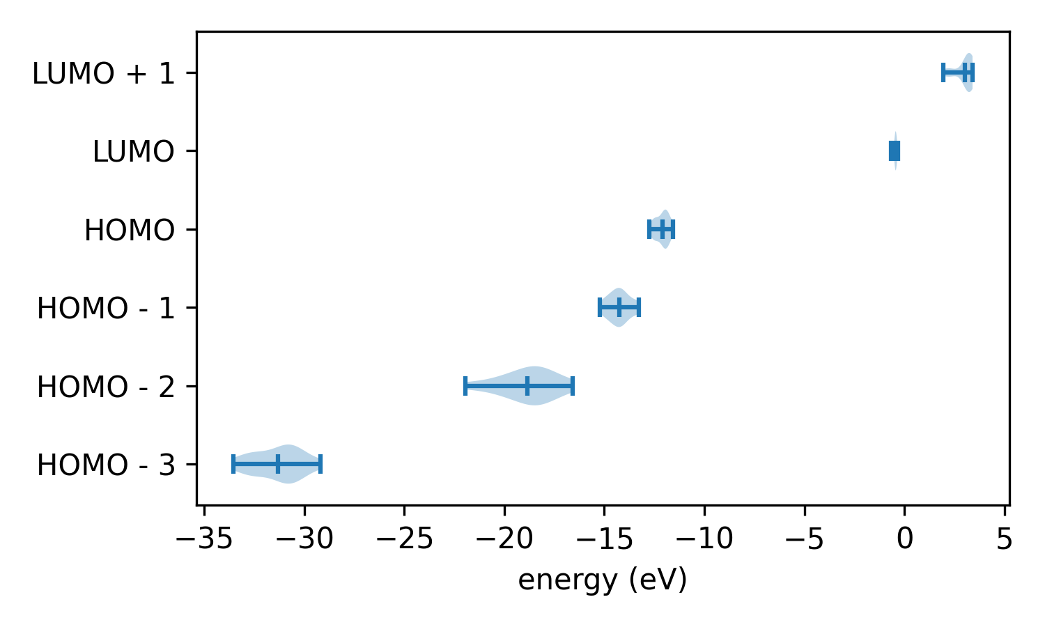
The distribution of the orbital energies across the screenshots (computed using machine-learned screening parameters)

Of course, these particular distributions don’t correspond to anything physical because the configurations were generated randomly. And furthermore, can we trust these results? We have skipped one important step: testing our model!

Testing the model

To test a model, we need to compare predicted screening parameters against those calculated ab initio. The input file for this task can be downloaded here. The key difference between this input file and the previous one is

        "from_scratch": true
    },
    "ml": {
        "test": true,
        "model_file": "../01-train/h2o_train_ml_model.pkl",
        "estimator": "ridge_regression",
        "descriptor": "orbital_density",
        "occ_and_emp_together": false,
        "n_max": 6,
        "l_max": 6,
        "r_min": 1.0,

Running this calculation, you will see the same output as in the previous calculation, but with the reappearance of the \(N \pm 1\) calculations that are required to calculate the screening parameters ab initio.

Calculate Screening Via DSCF
- Iteration 1
  - ✅ 01-ki completed
  - Power Spectrum Decomposition
    - Convert Orbital Files To XML
      - ✅ 01-bin2xml_total_density completed
      - ✅ 02-bin2xml_occ_spin_0_orb_1_density completed
      - ✅ 03-bin2xml_occ_spin_0_orb_2_density completed
      - ✅ 04-bin2xml_occ_spin_0_orb_3_density completed
      - ✅ 05-bin2xml_occ_spin_0_orb_4_density completed
      - ✅ 06-bin2xml_emp_spin_0_orb_5_density completed
      - ✅ 07-bin2xml_emp_spin_0_orb_6_density completed
    - ✅ 02-extract_coefficients_from_xml completed
    - ✅ 03-compute_power_spectrum_orbital_1 completed
    - ✅ 04-compute_power_spectrum_orbital_2 completed
    - ✅ 05-compute_power_spectrum_orbital_3 completed
    - ✅ 06-compute_power_spectrum_orbital_4 completed
    - ✅ 07-compute_power_spectrum_orbital_5 completed
    - ✅ 08-compute_power_spectrum_orbital_6 completed
  - Orbital 1
    - ✅ 01-dft_n-1 completed
  - Orbital 2
    - ✅ 01-dft_n-1 completed
  - Orbital 3
    - ✅ 01-dft_n-1 completed
  - Orbital 4
    - ✅ 01-dft_n-1 completed
  - Orbital 5
    - ✅ 01-dft_n+1_dummy completed
    - ✅ 02-pz_print completed
    - ✅ 03-dft_n+1 completed
  - Orbital 6
    - ✅ 01-dft_n+1_dummy completed
    - ✅ 02-pz_print completed
    - ✅ 03-dft_n+1 completed
  α
  
  1
  
  2
  
  3
  
  4
  
  5
  
  6
  
  0
  
  0.6
  
  0.6
  
  0.6
  
  0.6
  
  0.6
  
  0.6
  
  1
  
  0.493417
  
  0.576716
  
  0.560552
  
  0.492911
  
  0.463213
  
  0.578981
  
  predicted α
  
  1
  
  2
  
  3
  
  4
  
  5
  
  6
  
  0
  
  0.491291
  
  0.576154
  
  0.560565
  
  0.491663
  
  0.447122
  
  0.608699
  
  ΔE_i - λ_ii (eV)
  
  1
  
  2
  
  3
  
  4
  
  5
  
  6
  
  0
  
  0.991671
  
  0.190919
  
  0.346885
  
  0.999876
  
  -0.223314
  
  -0.0793481

We can compare the results using the accompanying python script, which extracts the orbital energies from the .pkl file and generates the following plot

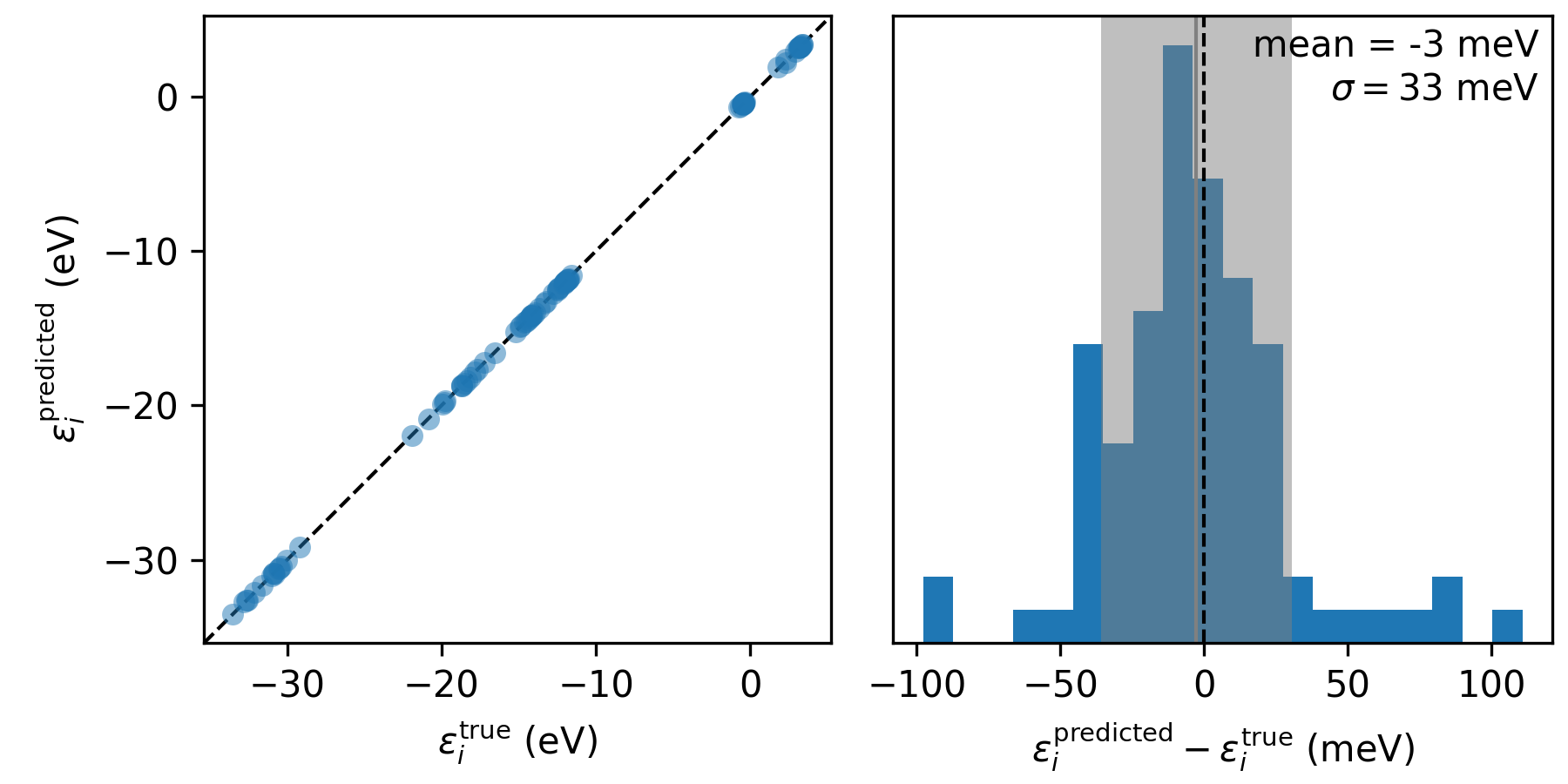
the accuracy of the orbital energies when using machine-learned screening parameters — The accuracy of the orbital energies when using machine-learned screening parameters (\(\varepsilon_i^\mathsf{predicted}\)) relative to those calculated ab initio (\(\varepsilon_i^\mathsf{true}\)) across the 15 test configurations.

Now we can understand the accuracy of our model: we can expect the orbital energies to be predicted within 40 meV or so of the ab initio Koopmans result. This is pretty good, given how rudimentary the model is and how little training it required!

Note

To really get a sense for the accuracy of this model, try and compare it to the accuracy you achieve when using an average screening parameter for all of the orbitals (set estimator to mean and then re-train and re-test).

More advanced testing (extra for experts)

So far, all of these tasks have relied on the pre-built workflows in the koopmans package. However, it is possible to use python to perform much more bespoke workflows. In the script provided in the final part of this tutorial, this functionality is leveraged to perform a convergence test on the accuracy of the machine-learning model as the number of training snapshots is increased.

For more details, refer to the script itself. Running the script generates the following plot

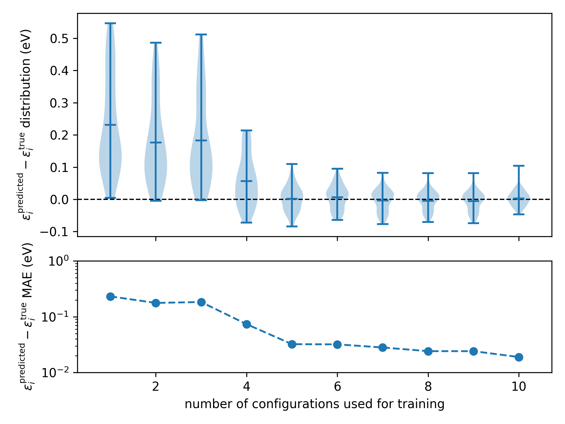
The accuracy of the machine-learning model as a function of the number of configurations used during training

Here we can see after five training configurations the model is beginning to saturate.

	1	2	3	4	5	6
0	0.6	0.6	0.6	0.6	0.6	0.6
1	0.574716	0.56594	0.49966	0.499231	0.566399	0.54828

	1	2	3	4	5	6
0	0.6	0.6	0.6	0.6	0.6	0.6
1	0.493417	0.576716	0.560552	0.492911	0.463213	0.578981